BAM! Bayesian Anything Model: a foundation model for generative computational imaging

Alessio Spagnoletti^1*, Charlesquin Kemajou Mbakam^2*, Jonathan Spence², Andrés Almansa¹, Marcelo Pereyra²

¹Université Paris Cité, CNRS, MAP5 UMR 8145, Paris, France
²Heriot-Watt University, MACS & Maxwell Institute for Mathematical Sciences, Edinburgh, UK
^*Indicates Equal Contribution

Paper Code & weights arXiv

ObservationBAM DIV2K | SR ×4

AFHQ Gaussian deblurring: BAM posterior sample

ObservationBAM AFHQ | Gaussian deblurring

FFHQ JPEG (Q = 10): BAM posterior sample

ObservationBAM FFHQ | JPEG (Q = 10)

ObservationBAM FFHQ | Inpainting

Köhler Blind motion deblurring: observation

Köhler Blind motion deblurring: BAM posterior sample

ObservationBAM Köhler | Blind motion deblurring

ObservationBAM LSUN | Inpainting

ObservationBAM LSUN | SR ×4

One small network, many imaging problems, few steps. Drag the sliders to compare each observation (left) with a BAM posterior sample (right). A single 36M-parameter network, with the forward operator supplied at inference time, covers ×4 super-resolution (DIV2K, LSUN), Gaussian deblurring (AFHQ), inpainting (FFHQ, LSUN), non-linear JPEG restoration at Q = 10 (FFHQ) and blind motion deblurring (Köhler), all in 3 steps.

Abstract

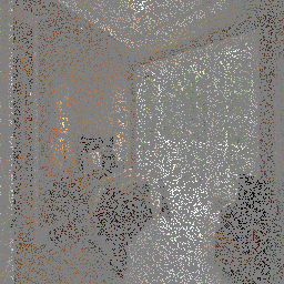
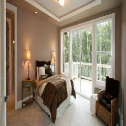
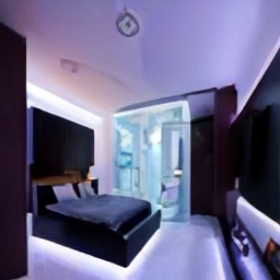
Generative models are transforming Bayesian computational imaging, yet the field still lacks physics-aware foundation models. Current practice falls into two camps. Large foundation image models are deployed as plug-and-play priors with zero-shot approximate likelihood guidance, which introduces significant bias and computational cost. Physics-aware generative models avoid this bias, but each is tied to a specific dataset, task and instrument. We introduce BAM (Bayesian Anything Model), a lightweight foundation model for few-step, physics-aware posterior sampling that generalises robustly to unseen data and tasks, zero-shot or with minimal finetuning. BAM upgrades the operator-conditioned Reconstruct Anything Model (RAM) backbone (Terris et al., 2025) into a conditional flow map, so instrument physics is specified at inference time rather than fixed during training. BAM has just 36M parameters and is pre-trained jointly on large image corpora and libraries of forward operators. A single network then draws posterior samples in a few steps, with no likelihood approximation and no guidance weights to tune. Across linear inverse problems on FFHQ, AFHQ, LSUN, DIV2K and the Köhler camera-shake benchmark, BAM outperforms in just 3 steps both specialised models and leading zero-shot methods in sample quality, at a fraction of their computational cost. BAM gives the community an accessible entry point to generative computational imaging, lowers the economic and environmental cost of training imaging models, and opens a new path for research on physics-aware Bayesian computational imaging. Code and weights will be released upon acceptance.

36M

parameters, one network for all problems

network evaluations per posterior sample

38/40

settings where a BAM variant has the best LPIPS

36/40

settings where a BAM variant has the best CMMD

Method

We consider imaging problems $y = A x^\star + \sigma_y w$, where the forward operator $A$ and the noise level $\sigma_y$ are known at inference time, and aim to draw samples from the posterior $p(\bm x \mid y, A, \sigma_y)$ in a handful of network evaluations. BAM is a conditional flow map: it transports a Gaussian reference $\rho_1 = \mathcal N(0, \sigma_d^2 \Id)$ to the posterior $\rho_0 = p(\bm x \mid y, A, \sigma_y)$, jumping between any two times $t \geq s$ of the probability-flow ODE. It amortises over a wide family of operators and noise levels, so a single model serves the whole family, with no retraining, or at most light finetuning, when the forward model changes.

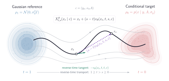
Schematic of the BAM conditional flow map — The conditional flow map $X^\theta_{t,s}$ moves a point from time $t$ to $s \le t$ along the probability flow that carries the Gaussian reference ($t=1$) to the posterior ($t=0$), with conditioning $c = (y_\sigma, \alpha_\sigma A)$. The purple arrow is the finite jump $(s-t)\,v_\theta(x_t, t, s, c)$; the green arrow is the reverse-time tangent $-v_\theta(x_t, t, t, c)$. Paths and densities are illustrative.

Physics-aware conditioning

Feeding $(y, A, \sigma_y, t, s)$ directly to a small network is numerically fragile, as $\sigma_y$ and $(t,s)$ span several orders of magnitude. BAM therefore conditions on a rescaled measurement, defined through the stochastic interpolant

$$\bm y_\sigma = \alpha_\sigma A \bm x + \varsigma_\sigma \bm w, \qquad \varsigma_\sigma / \alpha_\sigma = \sigma,$$

so that $y$ is a realisation of $\bm y_\sigma$ at $\sigma = \sigma_y$ up to the known factor $\alpha_\sigma$. The flow map is parametrised as

$$X^\theta_{t,s}(x \mid y_\sigma, \alpha_\sigma A) = x + (s-t)\, v_\theta(x, t, s, y_\sigma, \alpha_\sigma A), \qquad 0 \le s \le t \le 1,$$

which enforces the boundary condition $X^\theta_{t,t}(x) = x$ by construction. The velocity $v_\theta$ is a RAM backbone (an operator-conditioned DRUNet with unrolled physics-aware updates) that receives the augmented measurement $[x_t\,;\, y_\sigma]$ and the stacked operator $[(1-t)\Id\,;\, \alpha_\sigma A]$ supplied at inference time; its two noise-level embeddings take $t$ and $s$. $\sigma_y$ enters only through the rescaling, which keeps the model lightweight.

Training: Lagrangian self-distillation

On the diagonal ($t = s$) the velocity is fitted to the interpolant slope, and off the diagonal ($s < t$) the endpoint derivative of the map is matched to the drift of an EMA teacher $\theta^-$ at the transported point:

$$\mathcal L_b(\theta) = \mathbb E\big\| v_\theta(\bm x_t, t, t, \bm y_\sigma, \bm A) - (\bm z - \bm x_0) \big\|_2^2, \qquad \mathcal L_{\mathrm{LSD}}(\theta) = \mathbb E\big\| \partial_s X^\theta_{t,s} - \sg\big[v_{\theta^-}(\hat{\bm x}_{t,s}, s, s, \bm y_\sigma, \bm A)\big] \big\|_2^2.$$

Images $\bm x$ are drawn from large image corpora and operators $\bm A$ from a library of forward models (super-resolution, Gaussian and motion blur, compressed sensing, inpainting, demosaicing) with $\sigma_y \in [0, 0.05]$. The measurement noise is tied to $t$ through $\sigma(t) = \sigma_{\max}\gamma t / (1-(1-\gamma)t)$, which concentrates capacity where $\bm y_\sigma$ and $\bm x_t$ carry comparable noise. The full objective adds an LPIPS term and a contrast term, active only near $s \approx 0$:

$$\mathcal L(\theta) = \mathbb E\Big[\lambda_b \ell_b + \lambda_L \ell_{\mathrm{LSD}} + e^{-4s}\big\{\lambda_p \ell_{\mathrm{LPIPS}}(\hat{\bm x}_{t,s}, \bm x_0) + \lambda_c \ell_{\mathrm{ctr}}(\hat{\bm x}_{t,s}, \bm x_0)\big\}\Big].$$

No adversarial loss is used at any stage. Starting from the public RAM checkpoint, the baseline BAM is trained for 170 hours on 8 H100 GPUs; the fine-tuned variant BAM^★ continues for 16 hours on 2 H100 GPUs per target dataset, still across all problems.

Few-step posterior sampling

Each step re-noises the current iterate to level $t_k$, pairs it with a draw of the measurement interpolant at the matching level $\sigma_k = \sigma(t_k)$, and maps it back to $s = 0$ in a single network evaluation. Independent runs give independent posterior samples.

Algorithm 1: BAM posterior sampling (3 steps)

Given measurement $y$, operator $A$, noise level $\sigma_y$, schedule $1 = t_1 > t_2 > t_3$, levels $\sigma_k = \sigma(t_k)$, network $v_\theta$.
$\bm\varepsilon \sim \mathcal N(0, \Id)$ (held fixed across steps)
For $k = 1, 2, 3$
$\bm y_{\sigma_k} \gets \alpha_{\sigma_k} y + \sqrt{\varsigma_{\sigma_k}^2 - \alpha_{\sigma_k}^2 \sigma_y^2}\;\bm\varepsilon$ (add the missing measurement noise)
$\bm z^{(k)} \sim \mathcal N(0, \sigma_d^2 \Id)$
$\bm x_{t_k} \gets (1-t_k)\,\hat{\bm x}^{(k-1)} + t_k\, \bm z^{(k)}$ (pure noise when $t_1 = 1$)
$\hat{\bm x}^{(k)} \gets \bm x_{t_k} - t_k\, v_\theta(\bm x_{t_k}, t_k, 0, \bm y_{\sigma_k}, \alpha_{\sigma_k} A)$ (one NFE: $X^\theta_{t_k,0}$)
Return $\hat{\bm x}^{(3)}$

For small $\sigma_y$ the last step is taken at $\sigma_3 = \sigma_y$, where no re-noising is needed. For large $\sigma_y$, BAM sets $\sigma_2 = \sigma_y$ and takes the last step at $\sigma_3 < \sigma_y$, drawing the interpolant by a Brownian bridge between $A\hat{\bm x}^{(2)}$ and the rescaled measurement.

Results

LPIPS versus reconstruction FLOPs for BAM and baselines

State-of-the-art quality at a fraction of the cost

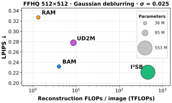
BAM advances the quality–cost Pareto frontier drawn by state-of-the-art methods: better perceptual quality (LPIPS) with fewer FLOPs per 512×512 image and far fewer parameters (bubble area). The same conclusion holds across metrics, inverse problems and datasets.

BAM is also robust to post-training quantisation: in INT8 under TensorRT it restores a 512×512 image in 80 ms instead of 281 ms on an NVIDIA A40 (3.5× faster), with a moderate loss in accuracy (PSNR −1.3 dB, LPIPS 0.400 → 0.427) and no fine-tuning after quantisation.

Reconstruction quality

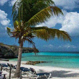
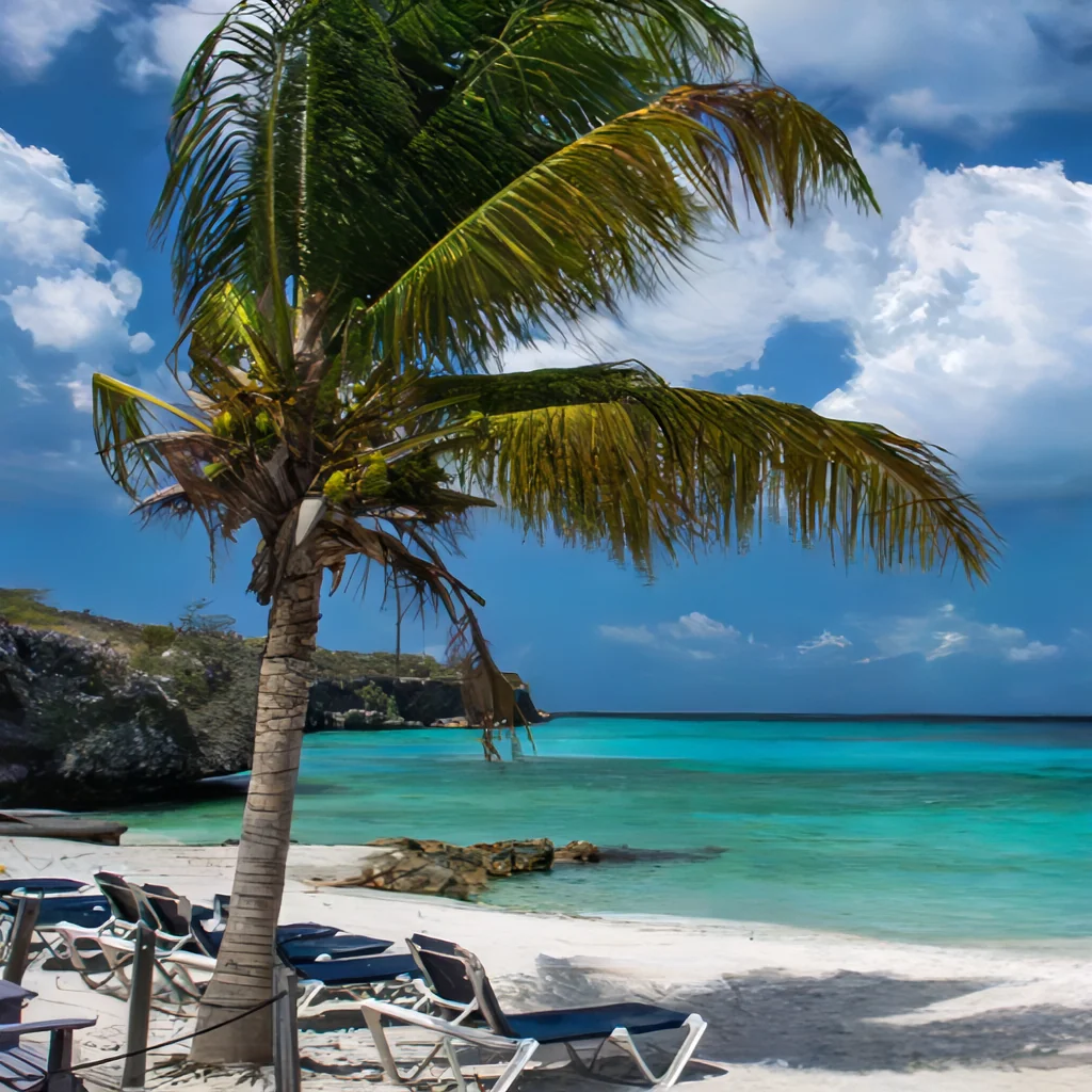
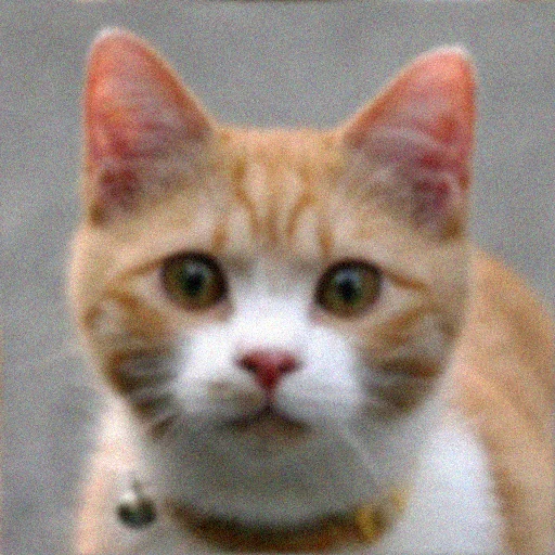
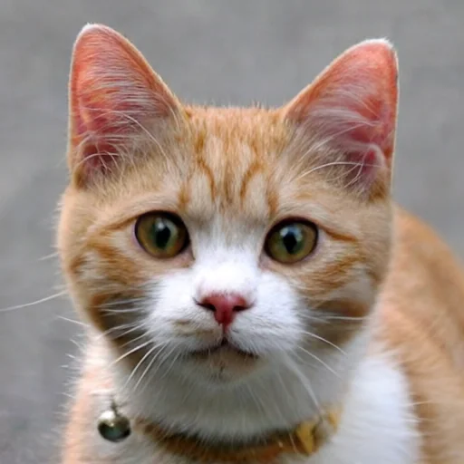
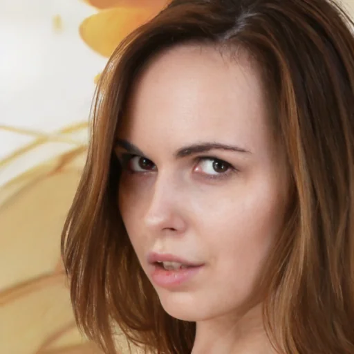
Across four datasets, five problems and two noise levels, a BAM variant attains the best LPIPS in 38 of 40 settings and the best CMMD in 36 of 40. BAM restores sharp, realistic textures such as fur, hair and foliage while remaining consistent with the measurements. RAM, trained as an MMSE estimator, often attains higher PSNR at the cost of smoother textures, while zero-shot and latent-space methods show noise artifacts or hallucinate content inconsistent with the observation.

DIV2K and FFHQ restoration at σ_y = 0.05

Method	NFEs	DIV2K				FFHQ
Method	NFEs	PSNR↑	LPIPS↓	CMMD↓	FID↓	PSNR↑	LPIPS↓	CMMD↓	FID↓
Gaussian deblurring
BAM	3	24.48	0.35	0.06	34.4	29.63	0.25	0.10	45.0
BAM^★	3	24.44	0.35	0.04	35.6	30.16	0.25	0.08	51.6
RAM	1	25.63	0.43	0.44	52.6	30.54	0.35	1.15	94.7
RAM^★	1	26.00	0.42	0.34	47.0	31.53	0.34	1.07	92.4
LATINO-PRO	65	23.55	0.54	0.49	71.9	23.40	0.46	1.17	128.3
SILO	200	17.20	0.62	1.84	298.8	24.92	0.38	0.25	91.8
I²SB	50	–	–	–	–	30.24	0.24	0.02	44.2
UD2M	12	–	–	–	–	29.30	0.29	0.72	67.3
Super-resolution
BAM	3	24.30	0.36	0.08	39.6	28.84	0.27	0.19	50.4
BAM^★	3	23.56	0.37	0.09	41.1	29.37	0.27	0.19	62.4
RAM	1	25.79	0.43	0.26	74.1	31.15	0.36	1.02	107.1
RAM^★	1	25.88	0.42	0.27	51.7	31.01	0.35	1.52	93.0
LATINO-PRO	65	22.82	0.54	0.59	95.3	23.18	0.53	0.90	146.3
SILO	200	16.53	0.64	2.04	308.4	25.04	0.37	0.20	80.7
I²SB	50	–	–	–	–	26.82	0.39	1.02	148.8
UD2M	12	–	–	–	–	28.16	0.31	0.30	82.2
Inpainting
BAM	3	26.61	0.27	0.02	20.5	31.50	0.23	0.08	32.1
BAM^★	3	25.66	0.27	0.03	21.0	31.57	0.20	0.05	32.4
RAM	1	23.52	0.41	0.30	66.9	25.55	0.39	1.53	126.5
RAM^★	1	27.61	0.32	0.18	35.5	32.40	0.29	1.12	56.5
LATINO-PRO	65	11.25	0.71	2.01	282.4	13.44	0.79	2.63	305.0
SILO	200	12.92	0.73	2.91	382.4	17.46	0.52	1.00	139.4
I²SB	50	–	–	–	–	18.89	0.58	1.93	174.2
UD2M	12	–	–	–	–	29.29	0.25	0.21	45.54

PSNR (dB, ↑), LPIPS (↓), CMMD (↓) and FID (↓). BAM variants use three steps; BAM^★ and RAM^★ denote finetuning. Bold and underline mark the best and second-best values for each dataset and problem; – denotes an unavailable result.

Visual comparisons

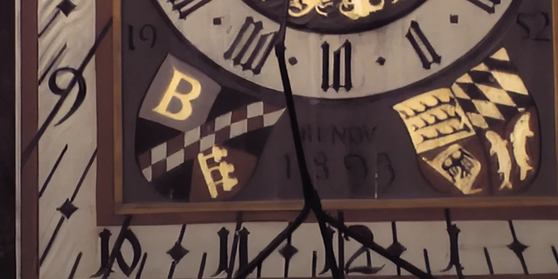
BAM and BAM^★ use three steps. Yellow boxes mark the region magnified 4× below each image. Click any image to compare it against another method with a slider.

DIV2K
FFHQ
AFHQ

Observation

BAM

BAM^★

RAM

RAM^★

SILO

TReg

Gaussian deblurring σ_y = 0.05

SR ×4 σ_y = 0.05

Inpainting σ_y = 0.05

Observation

BAM

BAM^★

RAM

RAM^★

SILO

UD2M

I2SB

FFHQ — Gaussian deblurring, σ_y = 0.05

FFHQ — SR ×4, σ_y = 0.05

FFHQ — JPEG, Q = 10, pre-compression σ_JPEG = 0.01

–

Observation

BAM

BAM^★

RAM

RAM^★

LATINO

L-PRO

TReg

SILO

AFHQ — Inpainting, σ_y = 0.05

AFHQ — Demosaicing, σ_y = 0.05

AFHQ — Compressed sensing, σ_y = 0.05

–

Full quantitative comparison

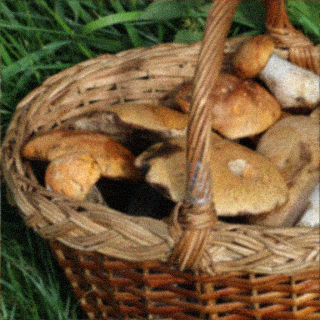
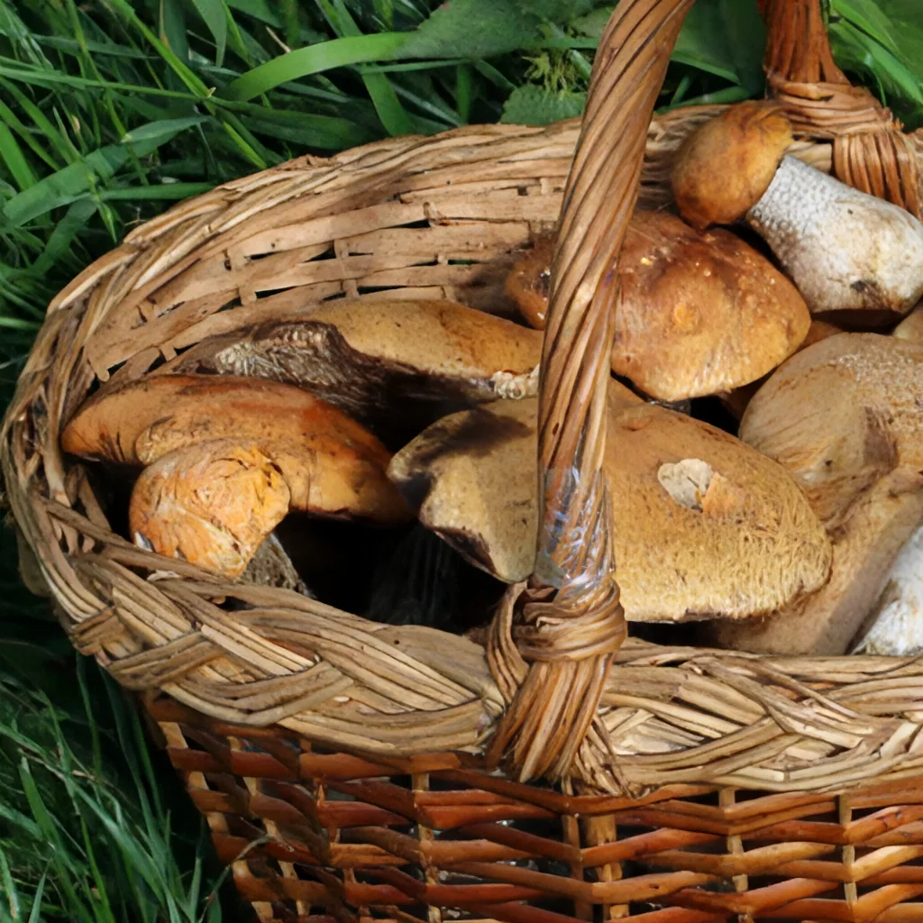
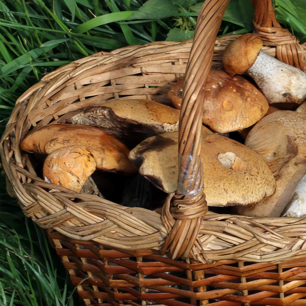
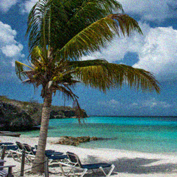
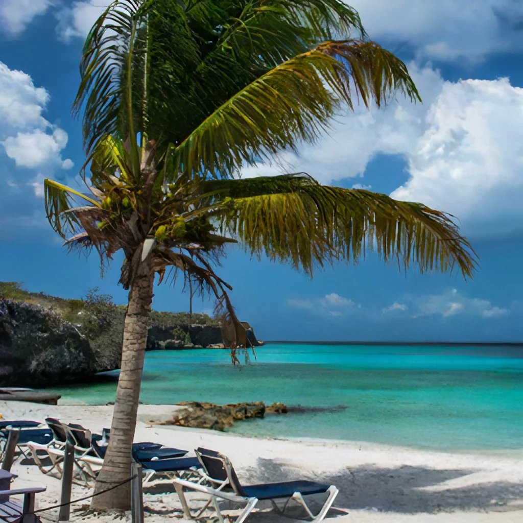
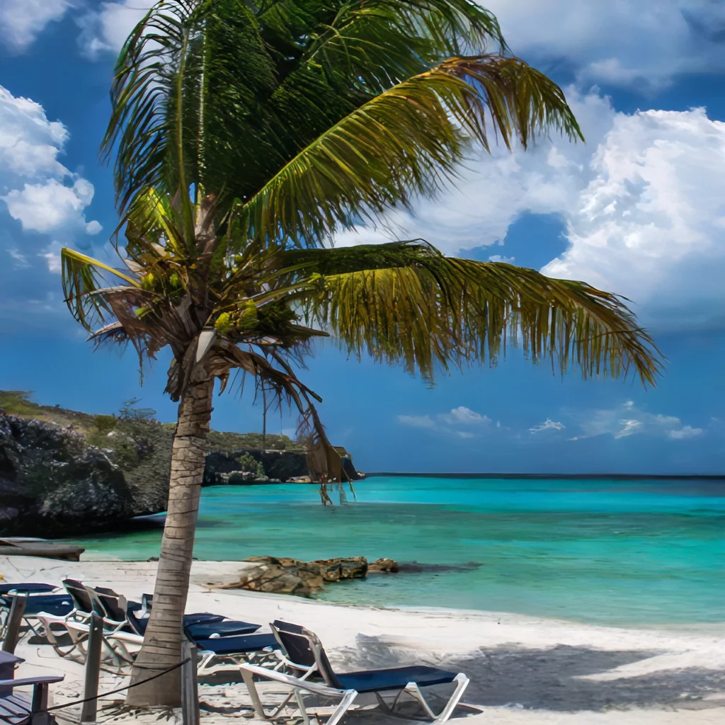
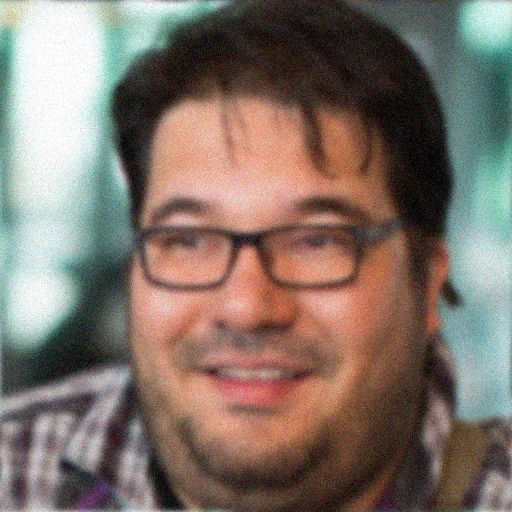
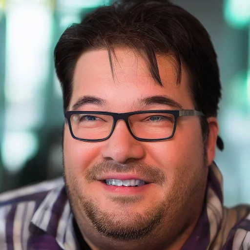
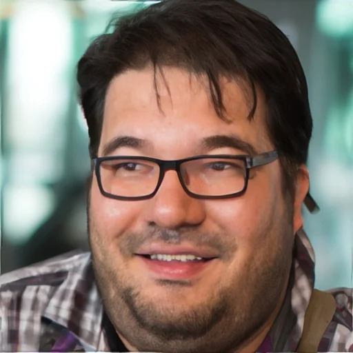
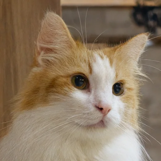
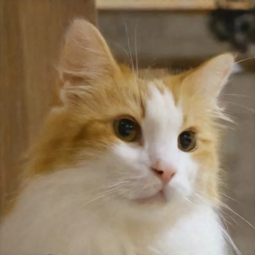
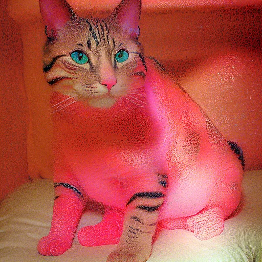
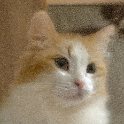
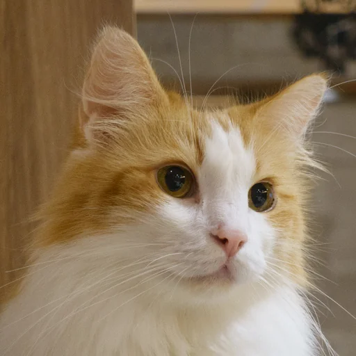
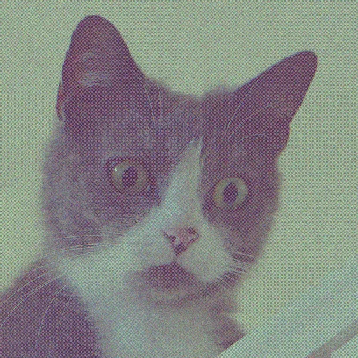
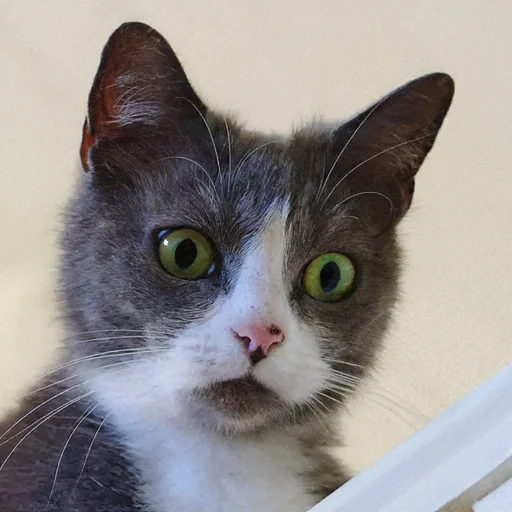
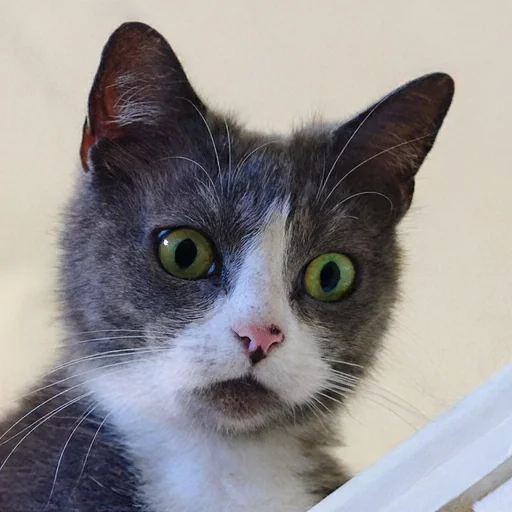
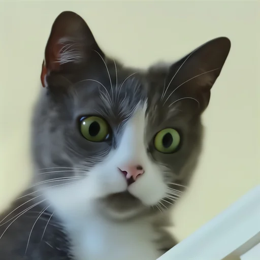
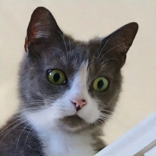
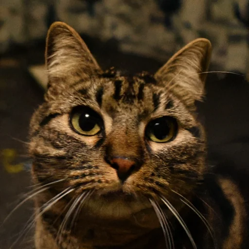
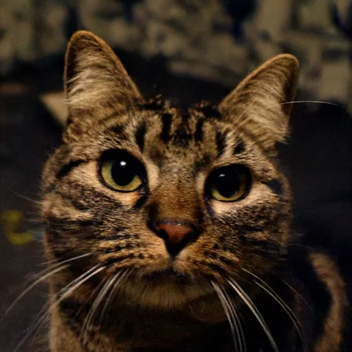
All five problems BAM is trained on, at σ_y ∈ {0.025, 0.05}. AFHQ and LSUN bedroom are out-of-distribution for the baseline BAM. PSNR (dB, ↑), LPIPS (↓), CMMD (↓), FID (↓); bold / underline: best / second-best value per problem, noise level and metric.

DIV2K
FFHQ
AFHQ
LSUN

DIV2K: 64 test images. BAM and BAM^★ use three steps.

Method	NFEs	σ_y = 0.025				σ_y = 0.05
Method	NFEs	PSNR↑	LPIPS↓	CMMD↓	FID↓	PSNR↑	LPIPS↓	CMMD↓	FID↓
Deblurring
BAM	3	25.01	0.334	0.04	33.51	24.48	0.349	0.06	34.43
BAM^★	3	24.91	0.339	0.03	33.80	24.44	0.353	0.04	35.59
RAM	1	26.08	0.401	0.37	41.35	25.63	0.427	0.44	52.55
LATINO	8	23.29	0.473	0.28	74.62	22.00	0.514	0.39	100.27
LATINO-PRO	65	24.07	0.454	0.35	66.02	23.55	0.536	0.49	71.90
TReg	200	22.43	0.485	0.34	83.89	21.85	0.515	0.40	102.21
SILO	200	17.56	0.614	1.72	287.03	17.20	0.624	1.84	298.80
Super-resolution
BAM	3	24.92	0.343	0.06	36.80	24.30	0.362	0.08	39.55
BAM^★	3	24.19	0.354	0.06	36.95	23.56	0.373	0.09	41.12
RAM	1	26.49	0.397	0.20	50.92	25.79	0.430	0.26	74.12
LATINO	8	24.36	0.478	0.37	57.15	22.70	0.542	0.56	97.24
LATINO-PRO	65	24.49	0.476	0.38	54.11	22.82	0.543	0.59	95.31
TReg	200	22.07	0.497	0.39	76.52	20.73	0.565	0.55	112.77
SILO	200	17.04	0.631	1.99	295.67	16.53	0.641	2.04	308.43
Inpainting
BAM	3	27.31	0.224	0.01	17.35	26.61	0.267	0.02	20.46
BAM^★	3	26.56	0.233	0.02	17.73	25.66	0.272	0.03	21.01
RAM	1	23.61	0.399	0.29	61.78	23.52	0.412	0.30	66.93
LATINO	8	15.22	0.692	1.74	229.43	14.45	0.704	1.76	224.50
LATINO-PRO	65	13.73	0.678	1.79	270.42	11.25	0.706	2.01	282.41
TReg	200	15.15	0.727	1.47	287.30	14.48	0.748	1.67	299.14
SILO	200	13.08	0.724	2.85	378.42	12.92	0.729	2.91	382.44
Demosaicing
BAM	3	33.37	0.121	0.01	7.38	30.48	0.194	0.02	12.68
BAM^★	3	32.61	0.127	0.01	8.51	29.85	0.196	0.02	14.02
RAM	1	30.09	0.341	0.20	53.56	28.75	0.385	0.26	70.95
LATINO	8	18.08	0.578	1.52	199.76	15.26	0.642	1.88	263.70
LATINO-PRO	65	18.58	0.531	1.28	163.41	15.42	0.610	1.67	248.64
TReg	200	19.57	0.529	0.38	101.76	18.28	0.594	0.59	135.35
SILO	200	14.92	0.717	3.19	380.73	14.63	0.723	3.00	389.20
Compressed sensing
BAM	3	30.63	0.172	0.01	12.86	28.87	0.221	0.02	16.84
BAM^★	3	30.22	0.181	0.02	13.73	28.36	0.230	0.03	18.48
RAM	1	23.39	0.386	0.35	42.74	23.20	0.422	0.47	49.31
LATINO	8	16.08	0.660	2.18	250.92	13.71	0.700	2.24	249.40
LATINO-PRO	65	16.24	0.633	1.86	248.34	13.16	0.679	2.08	275.27
TReg	200	17.10	0.659	1.05	195.95	16.27	0.691	1.22	224.85

FFHQ: 64 test images. BAM and BAM^★ use three steps.

Method	NFEs	σ_y = 0.025				σ_y = 0.05
Method	NFEs	PSNR↑	LPIPS↓	CMMD↓	FID↓	PSNR↑	LPIPS↓	CMMD↓	FID↓
Deblurring
BAM	3	30.63	0.232	0.09	40.63	29.63	0.250	0.10	44.98
BAM^★	3	31.17	0.225	0.08	47.33	30.16	0.245	0.08	51.61
RAM	1	31.07	0.327	0.94	83.37	30.54	0.351	1.15	94.74
RAM^★	1	32.31	0.316	0.85	82.58	31.53	0.341	1.07	92.38
LATINO	8	25.08	0.377	0.62	100.28	22.72	0.428	0.85	119.48
LATINO-PRO	65	25.89	0.395	0.82	111.25	23.40	0.456	1.17	128.26
TReg	200	25.16	0.394	0.82	112.07	24.28	0.422	0.73	117.41
SILO	200	25.80	0.372	0.38	92.87	24.92	0.375	0.25	91.84
I²SB	50	31.20	0.221	0.01	36.82	30.24	0.240	0.02	44.21
UD2M	12	29.39	0.278	0.83	65.87	29.30	0.288	0.72	67.39
Super-resolution
BAM	3	29.99	0.249	0.13	45.48	28.84	0.272	0.19	50.42
BAM^★	3	30.48	0.247	0.13	56.46	29.37	0.268	0.19	62.38
RAM	1	32.49	0.322	0.60	87.48	31.15	0.358	1.02	107.12
RAM^★	1	32.36	0.313	0.86	80.55	31.01	0.352	1.52	93.02
LATINO	8	25.53	0.419	0.66	99.47	22.18	0.510	1.13	141.33
LATINO-PRO	65	26.67	0.425	0.58	107.27	23.18	0.529	0.90	146.27
TReg	200	24.35	0.447	0.63	103.75	22.28	0.518	0.80	122.72
SILO	200	26.12	0.333	0.20	71.76	25.04	0.371	0.20	80.74
I²SB	50	26.20	0.387	1.11	151.20	26.82	0.393	1.02	148.82
UD2M	12	29.63	0.277	0.18	97.69	28.16	0.305	0.30	82.25
Inpainting
BAM	3	32.90	0.174	0.04	21.30	31.50	0.228	0.08	32.09
BAM^★	3	32.93	0.165	0.04	24.69	31.57	0.201	0.05	32.40
RAM	1	25.59	0.399	1.97	148.63	25.55	0.386	1.53	126.45
RAM^★	1	33.36	0.249	0.77	43.27	32.40	0.288	1.12	56.50
LATINO	8	13.98	0.773	3.25	247.94	13.43	0.776	3.27	248.21
LATINO-PRO	65	13.87	0.780	2.53	272.34	13.44	0.789	2.63	304.99
TReg	200	14.46	0.742	2.71	224.36	13.74	0.756	2.80	237.75
SILO	200	18.55	0.497	0.87	133.55	17.46	0.517	1.00	139.38
I²SB	50	22.38	0.491	1.35	134.48	18.89	0.584	1.93	174.26
UD2M	12	33.21	0.216	0.20	46.81	29.29	0.254	0.21	45.54
Demosaicing
BAM	3	36.45	0.119	0.03	10.95	33.38	0.202	0.05	23.77
BAM^★	3	36.49	0.114	0.04	12.70	33.94	0.167	0.04	19.25
RAM	1	31.95	0.333	0.57	101.48	30.78	0.370	0.66	110.64
RAM^★	1	37.36	0.161	0.34	18.74	35.07	0.226	0.46	32.27
LATINO	8	17.47	0.667	2.73	199.36	14.16	0.716	3.08	214.16
LATINO-PRO	65	18.19	0.635	1.76	170.99	13.12	0.743	2.08	255.00
TReg	200	21.15	0.547	1.37	125.35	18.87	0.626	1.78	159.45
SILO	200	20.26	0.510	1.43	137.00	21.04	0.472	0.85	118.79
Compressed sensing
BAM	3	34.58	0.151	0.03	16.37	32.41	0.208	0.06	25.52
BAM^★	3	34.91	0.145	0.03	19.17	32.72	0.185	0.04	25.02
RAM	1	24.47	0.411	1.17	75.17	24.35	0.461	1.21	88.65
RAM^★	1	33.74	0.262	1.13	41.35	32.72	0.301	1.29	54.27
LATINO	8	14.55	0.739	3.45	217.93	12.28	0.758	3.59	234.12
LATINO-PRO	65	14.73	0.743	2.68	232.97	10.75	0.823	3.04	322.00
TReg	200	16.60	0.690	1.95	168.07	15.46	0.717	2.29	197.12

AFHQ: 64 test images. BAM and BAM^★ use three steps.

Method	NFEs	σ_y = 0.025				σ_y = 0.05
Method	NFEs	PSNR↑	LPIPS↓	CMMD↓	FID↓	PSNR↑	LPIPS↓	CMMD↓	FID↓
Deblurring
BAM	3	27.41	0.336	0.23	33.52	26.89	0.354	0.26	35.62
BAM^★	3	26.85	0.294	0.18	23.89	26.41	0.311	0.19	24.21
RAM	1	27.85	0.417	1.17	52.11	27.46	0.444	1.41	60.40
LATINO	8	23.37	0.440	0.48	64.81	21.48	0.486	0.50	71.87
LATINO-PRO	65	24.62	0.494	1.44	67.77	22.63	0.558	1.60	92.28
TReg	200	23.49	0.469	0.89	76.62	22.74	0.497	0.93	81.11
SILO	200	24.43	0.420	0.31	42.88	24.05	0.420	0.30	44.82
Super-resolution
BAM	3	27.24	0.348	0.29	34.66	26.52	0.371	0.42	39.53
BAM^★	3	26.40	0.308	0.25	26.26	25.68	0.332	0.31	29.22
RAM	1	28.72	0.404	0.85	56.29	27.95	0.442	1.17	67.87
LATINO	8	23.27	0.478	0.92	70.52	20.48	0.560	1.35	92.08
LATINO-PRO	65	25.31	0.483	1.29	63.49	22.47	0.577	1.67	104.06
TReg	200	22.85	0.493	0.93	65.46	21.09	0.553	1.09	76.40
SILO	200	24.60	0.383	0.25	35.20	23.75	0.419	0.26	39.93
Inpainting
BAM	3	29.32	0.223	0.07	16.09	28.41	0.277	0.13	21.87
BAM^★	3	29.15	0.209	0.08	14.33	27.98	0.257	0.12	19.36
RAM	1	24.73	0.419	1.11	66.55	24.68	0.427	1.00	62.86
LATINO	8	14.20	0.739	2.04	92.70	13.65	0.737	2.01	85.07
LATINO-PRO	65	13.30	0.796	2.61	293.10	12.37	0.817	2.93	329.01
TReg	200	14.09	0.750	2.33	104.17	13.47	0.762	2.25	100.78
SILO	200	20.09	0.585	0.71	64.51	19.49	0.631	1.05	71.92
Demosaicing
BAM	3	34.66	0.129	0.03	7.86	31.49	0.215	0.06	15.77
BAM^★	3	34.23	0.125	0.06	7.56	30.84	0.204	0.10	15.08
RAM	1	30.67	0.388	0.73	62.01	29.42	0.438	0.89	73.68
LATINO	8	17.06	0.650	2.35	105.73	13.91	0.703	2.38	101.36
LATINO-PRO	65	18.07	0.614	1.87	95.46	13.83	0.708	2.22	160.66
TReg	200	18.83	0.585	1.92	97.06	16.63	0.660	2.35	114.93
SILO	200	21.80	0.466	0.31	47.84	21.77	0.477	0.28	47.71
Compressed sensing
BAM	3	32.05	0.173	0.05	12.20	30.10	0.233	0.09	18.23
BAM^★	3	30.97	0.178	0.08	12.01	28.65	0.241	0.11	19.26
RAM	1	23.97	0.404	1.12	38.90	23.83	0.446	1.31	44.47
LATINO	8	14.71	0.700	2.16	89.67	12.48	0.716	2.25	85.35
LATINO-PRO	65	13.86	0.769	2.74	230.27	11.16	0.829	3.05	297.84
TReg	200	15.22	0.710	2.46	92.96	14.40	0.735	2.52	97.29

LSUN: 300 test images. BAM and BAM^★ use three steps.

Method	NFEs	σ_y = 0.025				σ_y = 0.05
Method	NFEs	PSNR↑	LPIPS↓	CMMD↓	FID↓	PSNR↑	LPIPS↓	CMMD↓	FID↓
Deblurring
BAM	3	25.78	0.154	1.86	89.35	25.38	0.160	2.15	90.52
BAM^★	3	26.16	0.155	1.02	49.41	25.79	0.160	1.26	48.28
RAM	1	25.97	0.213	1.92	77.53	25.58	0.239	2.20	87.09
RAM^★	1	27.25	0.304	1.87	76.90	26.59	0.333	2.11	86.54
COSIGN	2	24.74	0.215	1.08	43.40	24.60	0.230	1.43	44.41
UD2M	12	25.96	0.279	1.68	81.61	23.45	0.380	2.55	98.44
CM4AI	1	23.82	0.419	2.29	199.04	23.33	0.443	2.36	213.70
Super-resolution
BAM	3	25.67	0.160	2.07	95.97	25.13	0.170	2.38	100.50
BAM^★	3	25.69	0.150	1.08	47.80	25.13	0.160	1.38	49.74
RAM	1	21.13	0.525	2.48	163.48	20.83	0.577	3.44	200.71
RAM^★	1	27.09	0.302	1.80	73.45	26.27	0.342	2.20	88.81
COSIGN	2	21.73	0.245	2.45	113.81	20.75	0.370	2.90	160.95
UD2M	12	23.50	0.439	3.40	114.50	23.78	0.315	0.67	48.31
CM4AI	1	25.78	0.324	1.76	128.71	25.52	0.320	1.57	123.33
Inpainting
BAM	3	28.13	0.067	0.77	65.90	27.46	0.090	1.19	76.43
BAM^★	3	28.24	0.060	0.41	39.74	27.51	0.071	0.55	38.77
RAM	1	23.14	0.224	2.55	125.54	23.30	0.224	2.42	120.08
RAM^★	1	28.64	0.238	1.31	53.26	28.20	0.261	1.58	60.24
Demosaicing
BAM	3	34.41	0.028	0.40	40.88	31.55	0.067	0.59	53.57
BAM^★	3	34.66	0.023	0.29	27.67	31.66	0.048	0.38	27.71
RAM	1	30.10	0.152	1.31	69.66	28.96	0.182	1.60	79.74
RAM^★	1	35.17	0.114	0.43	21.45	32.91	0.161	0.61	33.69
Compressed sensing
BAM	3	31.90	0.044	0.49	49.93	30.08	0.071	0.75	60.07
BAM^★	3	32.34	0.037	0.32	29.84	30.46	0.053	0.41	29.36
RAM	1	22.65	0.205	2.31	109.29	22.58	0.238	2.58	135.76
RAM^★	1	29.81	0.246	1.69	53.40	29.21	0.271	1.91	62.45

Beyond natural images

Sparse-view CT. BAM extends to CT on LIDC-IDRI chest slices with 51 parallel-beam projections, a single-channel modality far from the natural images seen during pre-training. After finetuning on CT, three-step BAM samples recover fine lung vessels, and the pixelwise standard deviation over 64 draws concentrates on anatomical edges and vessels, at the same order of magnitude as the error of the posterior mean: a spatial uncertainty map at no extra training cost.

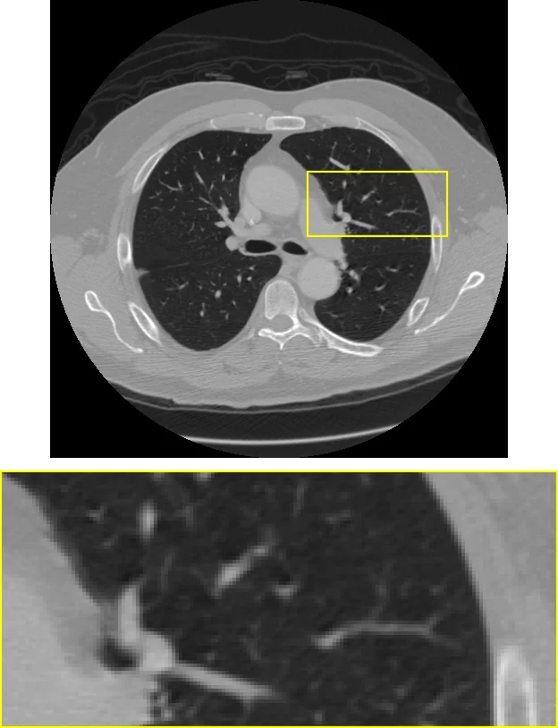
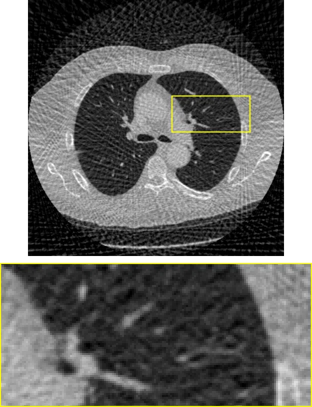
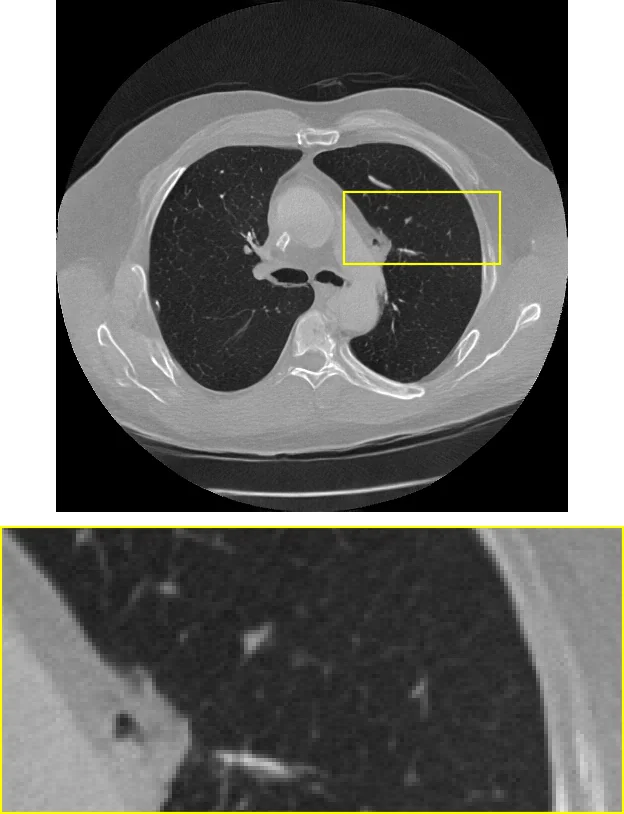
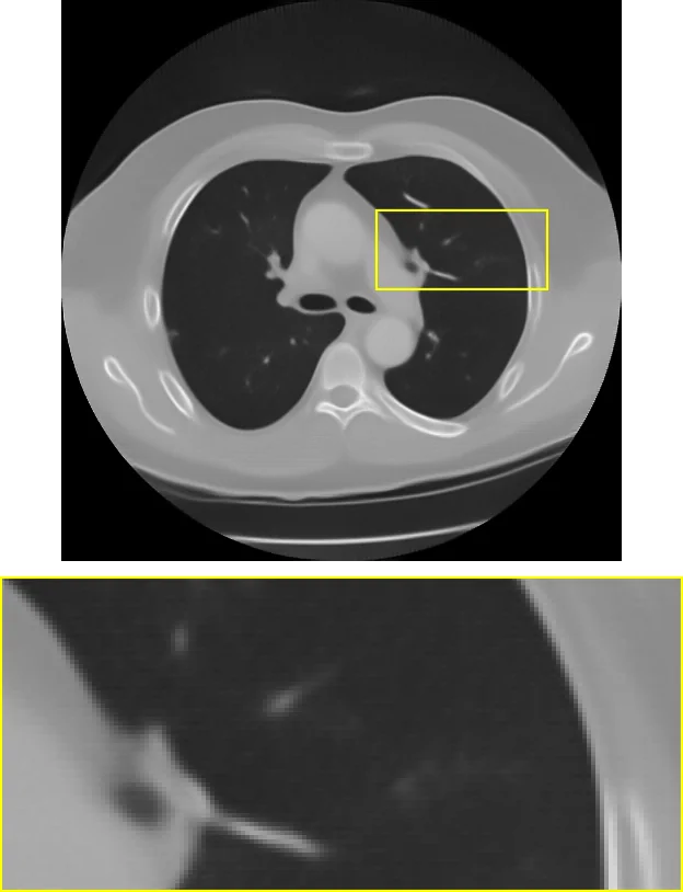
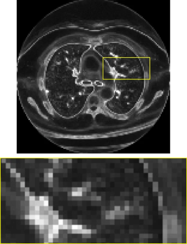
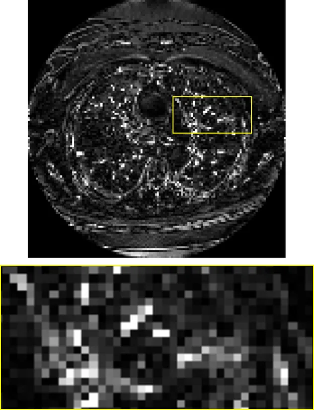
CT: Filtered backprojection — Filtered backprojection

CT: 4×4 std. (N = 64) — 4×4 std. (N = 64)

Left to right: ground truth, filtered backprojection, one BAM sample, posterior mean, standard deviation over 64 draws, and residual |GT − mean|. Yellow boxes and 4× strips show the same lung region in every panel.

Blind motion deblurring. With spatially varying kernels estimated by a pre-trained kernel predictor network, BAM outperforms both RAM and the original unrolled PnP architecture on the Köhler benchmark, although it was never trained on such operators.
Non-linear JPEG restoration. After finetuning, BAM restores noisy JPEG-compressed images (Q = 10), generating missing details and regularising noisy areas where zero-shot and unrolled methods generalise poorly.
Posterior mean. Averaging repeated BAM draws gives a Monte Carlo posterior-mean estimate whose PSNR exceeds that of the fine-tuned MMSE network RAM^★ on four of five problems: samples are sharp individually yet accurate on average.

Limitations

BAM handles only additive Gaussian noise and linear or mildly non-linear forward operators. It is non-blind, so blind problems rely on an external operator estimate. It does not detect model misspecification, so under strong distribution shift it can return unreliable posteriors without warning. Finally, posterior sample quality was assessed empirically; formal guarantees for the learned conditional flow map remain open.

BibTeX

@misc{spagnoletti2026bam,
  title  = {{BAM!} {B}ayesian {A}nything {M}odel: a foundation model for generative computational imaging},
  author = {Spagnoletti, Alessio and Kemajou Mbakam, Charlesquin and Spence, Jonathan and Almansa, Andr{\'e}s and Pereyra, Marcelo},
  year   = {2026}
}